Baby steps with Scilab

For me, the best way to learn a new programming language is by example. That, and figuring things out. Starting from an example code that creates a white circle on black background:

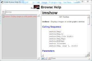
Try to figure out how each function work and what each line does. To make the guesswork easier, make friends with the language by learning how to ask for help. In Scilab, typing help _keyword_ or simply help opens the help window. Start by looking for the functions used in the example. I've already figured out what each line does and made comments. Comments are denoted by two slashes // and lasts for one line. Comments will not be interpreted and executed.

The sample program creates a circle and lets you view it using imshow. To be able to automatically save files, we can use the function imwrite. The following snippet let's you save the image produced from array A to a .jpg file on the path specified. You can choose what file format to use by changing the file extension, as long as it is supported by the function imwrite. See the imwrite help page for the list of supported formats.

The circle produced is centered and colored white in black background. As you may have figured out by now, the matrix A that produced this image is binary, with only 1's and 0's. The original matrix A, zeros(nx,ny) is black. The condition that all elements in A corresponding to the elements in r that are less than 0.7 be 1, makes the white circle. The image produced by imshow is grayscale with 0 being black and 1 being white.

circle.jpg

imwrite and imshow are special functions that came with the Scilab Image Processing (SIP) toolbox. Scilab toolboxes contain a set or sets of functions specialized for certain tasks like image processing. Functions in toolboxes will not work if it's toolbox is not loaded.

Now to play with the sample code. Try changing parts of the code and see what will happen. If you want to add a smaller black circle, add another condition:

annulus.jpg

If you want to make a different shape, look for the lines that makes the circle and modify. To make a square, I changed line 9 from the sample code to:

This produces a centered white square with side length defined by the variable side.

square.jpg

Modifying the first few line of the code this way:

I came up with:

roof.jpg

%pi is the constant pi or 3.1416... stored in Scilab.

The first three figures (circle, square, annulus) are actually images of apertures that can be used for simulating optical phenomena. The last one (the roof) is something we can use to make a figure that looks like a diffraction grating, by adding the condition:

grating.jpg

Now for a more challenging figure! A circular aperture with a Gaussian transparency. Try to visualize that first.

.

.

.

circular aperture with Gaussian transparency

That's just the same as the first circle, only that the center isn't purely white -- or that the elements of the matrix isn't just one or zero. The circle is shaded according to a 2-dimensional Gaussian function:

Well, it could be any function really. Or any aperture shape. You just have to set up the code for the aperture and the code for the shading, and combine the two. How to combine them to achieve the desired effect is the real question! And in comes the masking technique. Remember that the matrix that produces the image of the circular aperture contains only 1's and 0's, so that if we multiply this matrix to any matrix (of the same size, mind you) then we would retain the original values for those elements paired with 1 and nullify (to 0) those elements paired with 0.

And there you go! My first baby steps with Scilab shared with you. I hope you learned something, because I sure did. Don't hesitate to play around with the codes. Have fun figuring things out. :)

Ha! I'm giving myself a 10 for that Scilab lecture. XP

Equation for Gaussian function taken from: http://mathworld.wolfram.com/GaussianFunction.html