Pattern Recognition

Objects can be classified into a group/class in which they share almost the same features. To be able to classify an object belonging to one class, we must be able to extract certain features from it and compare this with a database of features of different classes. The features must be easily quantified. Comparison can be made using the minimum distance classification.

First, we compute for the mean features of a class by taking 5 images of objects belonging to one class and extracting features from it. The mean feature vector of a class is the matrix containing the average of the quantified features for the class.

I used four different objects (that is, four classes) with 5 training samples and 5 test samples.

 

Training sets for the coin, post, card, and leaf classes.

 From these, I extracted 7 features: the area from the binarized image, the means of the red layer, green layer, and blue layer, and the standard deviations of the red layer, green layer, and blue layer. Each feature was normalized to the maximum value for that feature from all the training images so that all features are equally considered. If it were not so, the standard deviations would not count at all compared to the pixel area of the images. We can now compute the mean feature vector from each class.

So now we examine different objects and classify them by determining the mean feature vector it is nearest to. 

Test objects.

 We can use the Euclidean distance

to determine the class. x is the feature vector of the test sample and m is the mean feature vector. The results are shown below. Each row indicates the test object and each column indicates the mean feature vector for the four classes. The values are the distances computed using the equation for the Euclidean distance. The minimum distance for each row would indicate the class to where the object belongs (highlighted in yellow). 

Everything was classified correctly yay! :D

___________________________________________________________________________

I'm giving myself a 10 for 100% correct classification. :D

Binary Operations

The morphological operations we have learned before can be put into better use with the opening and closing operations. The opening operation is so called because it can "open" up spaces in an image, while the closing operation can "close" spaces depending on the structuring element (strel) used. Both operations make use of the erode and dilate operations discussed in the previous post. Let's consider this 14x18 pixel image:

To apply the opening function using a 2x2 square strel, first apply erode on the image then apply dilate on the eroded image. The resulting opened image looks like

Do you see now why the function is called open? :)

The closing operation is just the opening operation in reverse. Dilate the image then erode the dilated image. Using the same 2x2 strel, the closed image looks closed! :D

Looking for cancer cells

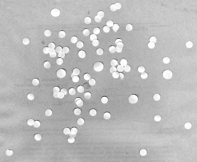
We can use the opening and closing operations to look for cancer cells (larger cells) in a pool of normal cells. Let's pretend that this image is an image of normal cells

normal cells

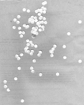
and this an image of normal cells with larger cancer cells

normal cells with cancer cells

The goal is to separate the cancer cells from the normal cells. First we have to differentiate the normal cells from the cancer cells. We can do this by first determining the area of normal cells.

First, I cut the image into 256x256 subimages and binarized the images. Choosing carefully the threshold to separate the background from the cells. By looking at the histogram of the grayed image, we were able to determine the threshold (~0.84).

Binarized subimages.

The opening operator is then applied to separate closely placed cells. The strel used is a 5x5-pixel circle with the center at the topmost left 1-valued pixel.

Opened subimages.

Using the bwlabel function in Scilab, we can separate each white cell or blob and compute for the area of each one using follow and Green's function (see post on Area Estimation). We get the mean and standard deviation of the areas computed. The first computation returned: mean =618.53968, standard deviation=184.75568. The large standard deviation is because of the areas that are too big or too small. These are the cells that overlapped to form big white blobs or the background noise that wasn't removed with thresholding. To get the best estimate of the area of the normal cells, we must remove the outliers. I did this by removing all blobs with areas that are less than the mean+standard deviation and those that are greater than the mean+standard deviation. We can loop this until we find a mean that doesn't change much after each iteration (less than 50 pixels for me). This means that the mean we computed is the "true" mean, without the outliers. After this process, we arrive at a mean of 443.91489 pixels and standard deviation 60.940662 pixels for the normal cells. 

With this, we may now look for cancer cells! Using the fact that the average area of a normal cell is ~ 444 pixels, we can make a circle with the same size and use this as strel to process the image of normal with cancer cells. First we binarize the image,

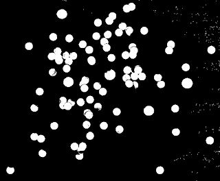
Binarized image of normal cells with abnormally large cancer cells.

Then, use the opening operation with the circular strel,

Applying the opening operation on the binarized image.

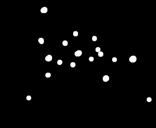
Do you see the cancer cells now? There are only 5 of them, but still too many normal cells here. Let's see if applying the opening operator again can remove these.

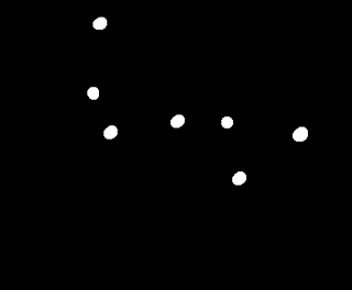
The opening operation applied twice.

Now there's the five cancer cells with two outliers. Not bad. :D

If we try to use the opening operation on this image again, we'll lose four of the cancer cells, leaving only one normal cell and one cancer cell. That's not good. Two dead normal cells are better that leaving the cancer cells behind undetected. 

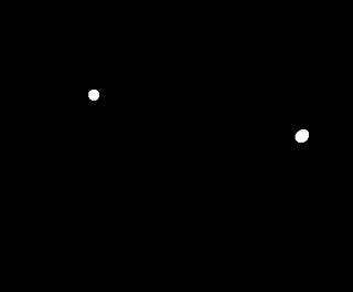
The opening operator applied thrice on the binarized image.

____________________________________________________________________________

I'm giving myself a 10 for this activity. I think I explained the opening and closing operations well enough and I liked how the rest of the blog went.

Morphological Operations

In this post, we will be looking at operations that morph an image systematically: erode, dilate, skel, and thin.

When we say morph, the shape of an object is transformed by using a structural element or a 'strel'. Usually a strel is a pattern made of a few number of pixels. The choice of strel depends on the desired effect on the image. Depending on the morphological operation and strel used, two objects in an image can be separated,
holes can be patched, noise pixels could be removed, among other effects.


Erode
The erosion of an object/shape A by a strel B is denoted by

Don't worry, that's not a very complicated mathematical expression. It's just set theory. In human langauage, that equation means that the erosion (that is, the image that will remain after the erosion operation) is the set of pixels where B could be placed so that it is still inside A. It is important to set a 'center' z (denoted by the circle in the figures below) for the strel. To erode a shape A, move the center of the strel B through each pixel of A. If the pixel in A cannot contain the whole strel, remove that pixel. The resulting image is a reduced version of the original.

Step-by-step erosion process.

Dilate
The dilation of an object/shape A by a strel B is denoted by

The concept is similar to erosion, move the center of the strel through pixels of the image and dilate. But this time, the strel has to be reflected (in x and y) first. See the reflected strell in the step-by-step procedure below. As you move the reflected strel through A, add the pixels outside A covered by the strel. The resulting image is a bloated version of the original.

Step-by-step dilation process.

In Scilab, erode and dilate can be implemented using the functions erode and dilate. Of course, that wasn't the first thing I did to learn how erode and dilate works! I posted the ones I did on graphing paper and the ones made using erode and dilate on Scilab. Examine how a square annulus, a plus sign, a square and a (somewhat) triangular shape are eroded and dilated by 5 different strels. The centers I used for the strels are denoted by an o. The shapes are marked with a red border. Shaded regions are the pixels removed, and squares with broken line borders are added pixels.

EROSION

The Strels.

Erosion of a 10x10 square annulus.

Erosion of a 5x5 plus sign.

Erosion of a 5x5 square.

Erosion of a 3x4 triangle.

DILATION

The Reflected Strels.

Dilation of a 10x10 square box.

Dilation of a 5x5 plus sign.

Dilation of a 5x5 square.

Dilation of a 3x4 triangle.

There are other functions in Scilab that can morph an image. The functions thin and skel were also used to morph the 4 shapes I used above (box, plus, square, triangle). These two functions are operations that thins the image and gives its skeleton both using different rules and algorithm for the thinning operation. 

_________________________________________________________________________________

I think I deserve a 10 for the nice illustrations and the effort into drawing all that. :D